Model Merging — a biased overview
A friendly tour of model merging, suspiciously aligned with my own research.

Motivation
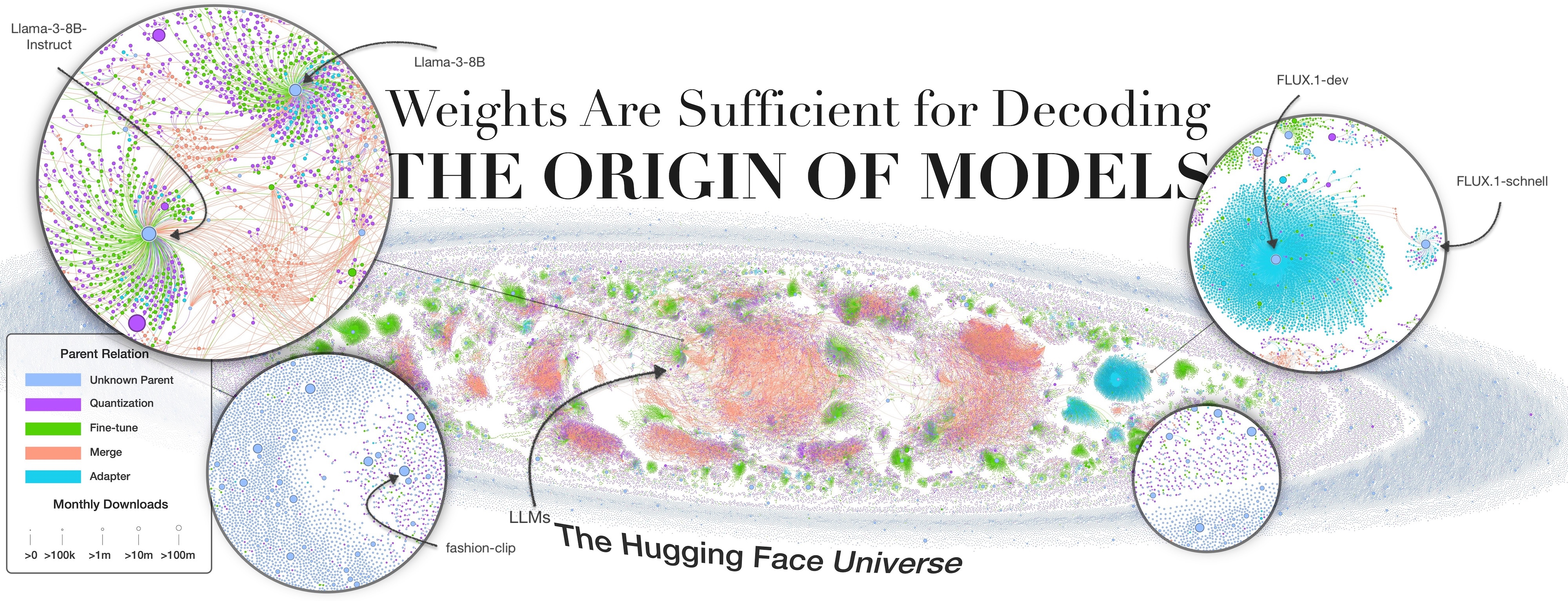
I recently attended an Estimathon game. This is basically a quiz where you estimate for some hard-to-quantify question like “How many cabs are there in New York?”
“How many models were there on HuggingFace one year ago?”
Take a moment to think before scrolling. Got your answer? Nice. Click to reveal the answer.
Number of models on HuggingFace last year 👀
Answer: 841,347 models.
Were you close? No? Okay, another chance:
“How many models are there on HuggingFace today?”
As above, think about it. You’re basically guessing the growth rate of HuggingFace itself.
Number of models on HuggingFace today 👀
Answer: 1,957,743 models.
Almost got it this time? Cool, you win a t-shirt or something. As you can see, the number has more than doubled in just one year!
With this explosion of models, a natural question comes up: should we keep making new ones, or spend more effort reusing what we already have? If, like me, you lean toward the latter in many practical cases, this blogpost is for you. Apparently, that’s also the view at Thinking Machines Lab (which just closed a $2B seed round), where they plan to “combine neural network layers from a range of open-source models with a technique that is similar to model merging”.
But even if you just want to make the GPUs go brrr and focus on training and tuning as much as possible, model merging might still be for you. ByteDance found merging effective for LLM pretraining
Enough motivation, let’s merge!
Intro to model merging
First things first, what is model merging? Informally, it’s any technique that, given two or more models (the endpoints) produces a new one that preserves their capabilities. Typically, we want the merging process to be data-free, and the resulting model to have:
- The same number of parameters as the endpoints.
- No extra runtime overhead.
These requirements are not always enforced. Depending on the use case, it might make sense to relax one of them — for example, allowing extra overhead for routing or using a small dataset to find better merging coefficients.
Okay, but what models are we merging, and why? It’s helpful to think in terms of two broad categories. The subdivision is not strict, but it makes the landscape easier to navigate:
- Merging models trained from scratch on the same task — covering linear mode connectivity, neuron permutation symmetries, and permutation matching.
- Merging models finetuned from the same base model on different tasks — including task vectors, structure-aware merging methods, and evolutionary merging of LLMs.
Merging models trained from scratch on the same task
The setup is simple: we start with two models initialized differently, $\theta^A_{\text{init}}$ and $\theta^B_{\text{init}}$. We train both on the same task $t$, then merge them into a new model $\theta_t^{A,B}$. Since the task index doesn’t add much information in this context, we drop it.
Mode connectivity
It all began with mode connectivity.
People once thought that parameters corresponding to different minima (modes) were isolated in the loss landscape, each mode living in its own valley (basin). This was bad news: if true, you couldn’t move between minima without incurring a sharp loss increase. But can these modes actually be connected in weight space via a low-loss (or high-accuracy) path?
Turns out the answer is yes:
- Yes, and this allows us to interpolate between them to obtain cheap ensembles
. - Yes, and in fact a large number of modes lie on a shared low-loss manifold
. - Yes, and if the two modes share an initial training phase, the connecting path may even be linear
.
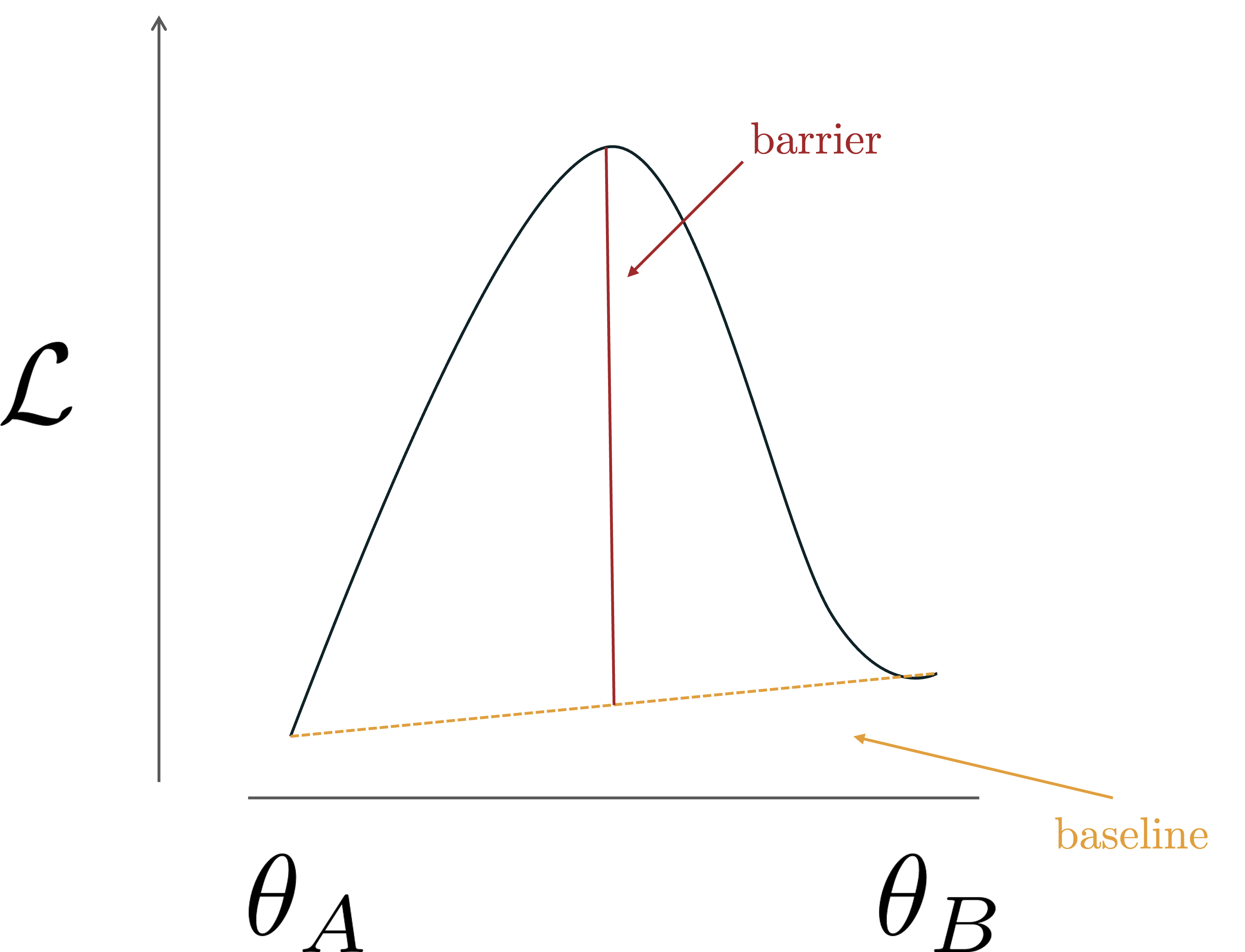
When the connecting path is linear, we usually assume the two modes to live in the same basin. This is kind of a big deal in model merging. Why? Well, because if the two modes can’t be connected linearly (i.e., linear interpolations between the modes result in a high loss), then we can’t average the models. Or, at least, can’t do it this simply. But how can we check if two modes are linearly connected, and to what degree? We will need to compute the loss barrier between the two.
\[\underbrace{\max_{\lambda \in [0,1]} \mathcal{L}\!\left((1-\lambda)\theta_A + \lambda \theta_B\right)}_{\text{highest loss along the path}} - \underbrace{\tfrac{1}{2}\Big(\mathcal{L}(\theta_A) + \mathcal{L}(\theta_B)\Big)}_{\text{average loss at endpoints}}\]Here, the first term measures the highest loss encountered along the linear interpolation between the two modes, while the second one is the average loss at the endpoints. If the two modes lie in the same basin, the interpolated loss remains low and the barrier is close to zero. A high loss barrier instead suggests the presence of a peak or saddle point separating the two modes, indicating they belong to different regions of the loss landscape.

Now that we know how to measure for closeness in the basin sense, we can move on to one of the key insights in model merging.
Neuron permutation symmetries
Consider a generic linear layer $z_{\ell+1} = \sigma(W_{\ell} z_{\ell})$, removing biases for simplicity. Now, what happens if we shuffle the rows of $W_{\ell}$? That’s equivalent to multiplying on the left by a permutation $P$, giving $W_\ell’ = P W_\ell$. The new output is
\[z'_{\ell+1} = \sigma(W_{\ell}' z_{\ell}) = \sigma(P W_{\ell} z_{\ell}) = P \sigma(W_{\ell} z_{\ell}) = P z_{\ell+1}.\]Here, we’ve pulled $P$ outside $\sigma$, possible because nonlinearities act elementwise and commute with permutations.
So far, the two networks (with $W_{\ell}$ vs $W’_{\ell}$) aren’t the same; their outputs differ by a permutation. But let’s also permute the columns of the next layer by $P^\top$. Since permutation matrices are orthogonal ($P^{-1} = P^\top$), the output of the next layer becomes:
\[z'_{\ell+2} = \sigma(W_{\ell+1}' z'_{\ell+1}) = \sigma(W_{\ell+1} P^\top P z_{\ell+1}) = \sigma(W_{\ell+1} z_{\ell+1}) = z_{\ell+2}.\]No tricks, the math checks out. The outputs are identical.
So, are these two networks the same? Internally, no, their weights differ (potentially a lot). But functionally, yes: they compute the exact same mapping.
This shows that neuron permutations create families of functionally equivalent networks. And since different random seeds lead to different permutations, many distinct-looking weight configurations are actually the same function.
This led to the conjecture: once you account for permutations, all modes collapse into a single shared basin torch.mean(A, B) is all you need!
Neuron matching
We wrapped up the previous section looking for a magical way to align the neurons of two models. One possible objective could be the following
\[\arg\max_{\{P_\ell \in \mathbb{P}\}} \sum_{\ell=1}^{L} \left\langle W_\ell^A, \, P_\ell W_\ell^B P_{\ell-1}^{\top} \right\rangle\]where
\[\langle A, B \rangle = \mathrm{tr}(A^\top B) = \sum_{i=1}^m \langle A_{i,:}, B_{i,:} \rangle,\]so at layer $\ell$ we are basically looking for the permutation $P_{\ell}$ that best aligns the rows (neurons) of the two matrices in a dot product sense. $P_{\ell}$ is then also applied, after transposition, to the subsequent layer to maintain functional equivalence.
Like all good things in life, this problem is NP-Hard
def match_neurons(A, B):
    # Initialize permutations as identity
    P = [identity(N) for l in layers]

    for i in num_steps:
        progress = False
        for l in shuffle(layers):

            W_A, W_B = A[l], B[l]

            # Compute neuron-to-neuron similarity matrix under current permutation
            sim = compute_similarity(W_A, P[l] @ W_B @ P[l-1])

            # Solve linear assignment problem
            new_P_l = linear_assignment_problem(sim)

            # Update permutation
            P[l] = new_P_l

            # Recompute similarity
            sim_new = compute_similarity(W_A, P[l] @ W_B @ P[l-1])

            if sim_new.mean() > sim.mean():
                progress = True

        if not progress:
            return P
Surprisingly, while Git Re-Basin (2022) is probably the most popular matching algorithm, a precursor (and also, a general case) of this algorithm by S.P. Singh and M. Jaggi was already around in 2019!
so each row/column has exactly one 1 (hard assignment), while a soft map may look like
\[\textbf{Soft map } S = \begin{bmatrix} 0.7 & 0.3 & 0.0 \\ 0.2 & 0.5 & 0.3 \\ 0.1 & 0.2 & 0.7 \end{bmatrix}\]so rows/columns sum to 1, entries in $[0,1]$ (fractional assignment). Soft maps are the bread and butter of optimal transport.
Entering cycle-consistency
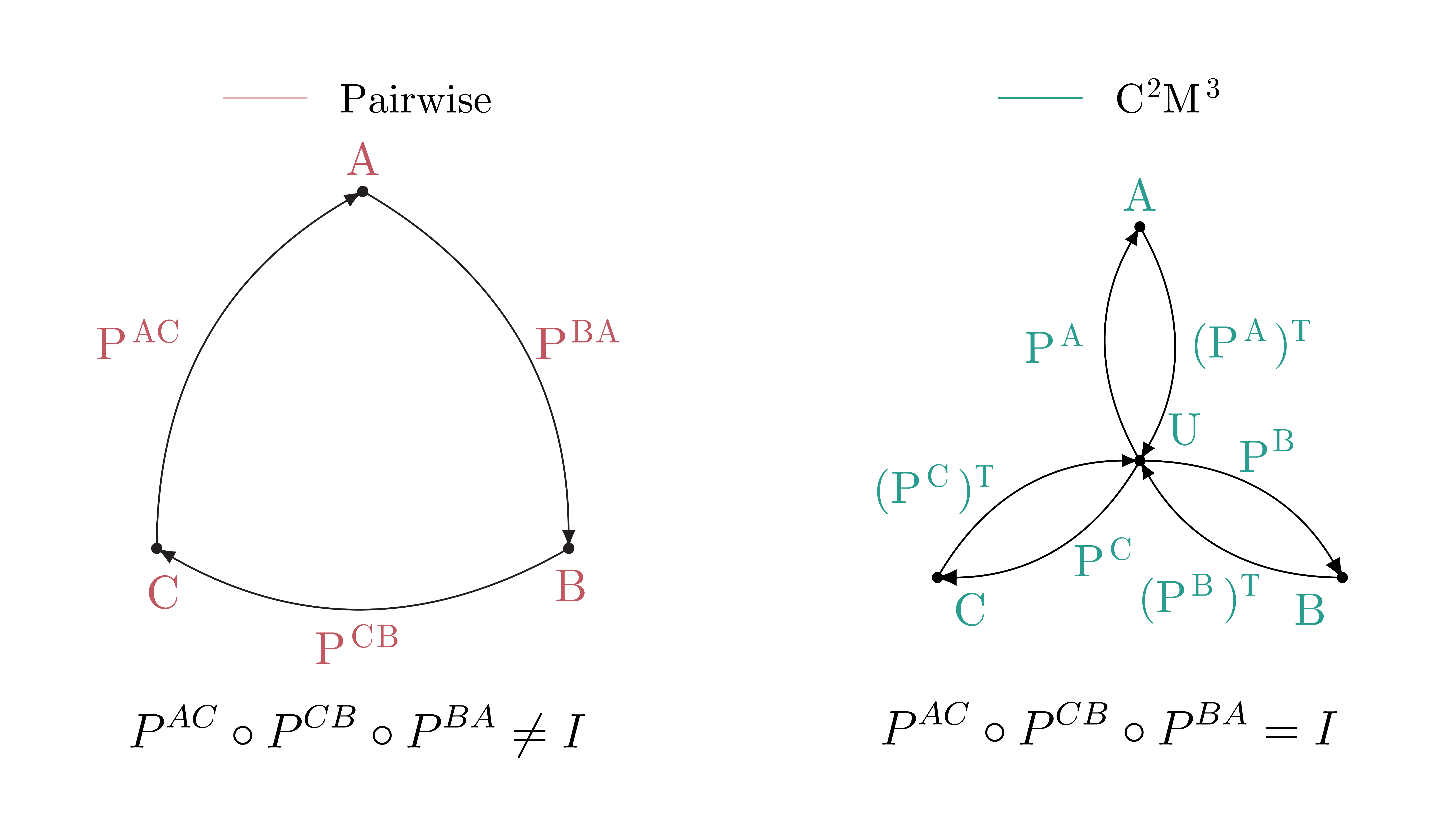
Now entering my own work: I’ll try to keep it fair and high level, so I don’t monopolize the overview. I can do this. The question here is: what happens if we want to match and merge more than 2 models? The easiest solution would be to choose one reference model, find pairwise maps to it, and then aggregate everything in this one. Couple of problems: when optimizing for each pair, the optimization is not aware of the other models. This means that the maps do not compose gracefully: if one maps from a model A to B, then to C and back to A, the end result would be way different than the starting point. In other words, the maps lack cycle-consistency. The other (main) problem is that the reference model is an arbitrary choice. And we know, arbitrariness is never good as it opens the way to variance in the results: depending on a (often random) choice might change the results by double digits. Let’s try something else! In $C^2M^3$
We factorize each permutation $P^{BA}$ (mapping $A$ to $B$) as the composition of two permutations: one mapping $A$ to a universe space, and one mapping from the universe back to $B$. Since each time you have to pass through the universe, you end-up with a series of permutations that cancel each other out, eventually composing to the identity and guaranteeing cycle-consistency.

The optimization problem we obtain is similar, just a tiny bit uglier due to the factorizations. We optimize this one with Frank-Wolfe

Merging models finetuned from the same base model on different tasks
We now switch setup. Tabula rasa. This time we start from a common pretrained model $\theta_{\text{pt}}$, which is finetuned separately on different tasks $t_1, t_2$ (say, MNIST and CIFAR-100) to obtain $\theta_{t_1}$ and $\theta_{t_2}$. Our goal is to combine them into a single model $\theta_{t_1,t_2}$ that:
- Has the same number of parameters as the base.
- Can do both tasks at once.
As before, we want this merging process to be data-free. Picture downloading two finetuned checkpoints from HuggingFace and fusing them into a single multi-task model without touching the original datasets.
So how do we do it?
Task arithmetic
The story begins with a simple yet powerful observation: finetuning on a task looks like adding a vector in weight space. This is trivially true when you consider the difference between the finetuned model and its base. Let us denote the update induced by task $t$ as the task vector
\[\tau_t = \theta_t - \theta_{\text{pt}}.\]Then, finetuning is nothing more than
\[\theta_t = \theta_{\text{pt}} + \tau_t.\]This way of writing things suggests an almost irresistible idea: if we want a model that can do both $t_1$ and $t_2$, why not just add their updates?
\[\theta_{t_1,t_2} = \theta_{\text{pt}} + \tau_{t_1} + \tau_{t_2}.\]And there you have it: task arithmetic
Of course, life isn’t quite that easy. Sometimes adding updates works beautifully, sometimes it leads to catastrophic interference, and sometimes you get a weird in-between model that can’t do either of the tasks. Still, the arithmetic view was an important first step: it made explicit that task updates behave vectorially, and therefore can be combined, compared, and even algebraically manipulated.
So, in general, merging models through task arithmetic boils down to
\[\theta_{\text{MT}} = \theta_{\text{pt}} + \alpha \sum_{t \in T} \tau_t\]where $\alpha$ is a scaling factor that is usually optimized on a validation set.
Task vectors and gradients
When I first heard about task arithmetic, I was puzzled: why should adding two random finetuning updates give anything meaningful? Let’s do a simple thought experiment.
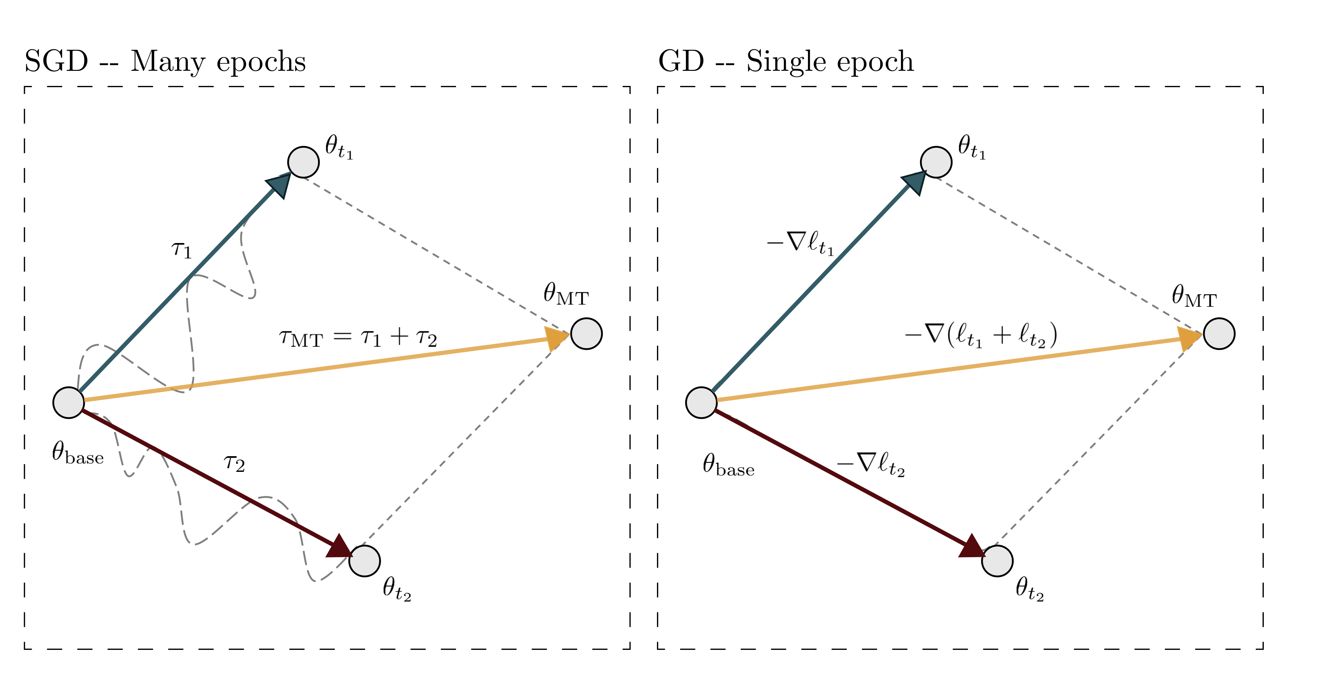
Suppose you finetune a pretrained model with vanilla gradient descent, no minibatches, and only a single epoch. In this case, the task vector is exactly the negative gradient of the loss at the base model:
\[\tau_t = - \eta \, \nabla \overline{\mathcal{L}}_t(\theta_{\text{pt}}),\]where $\eta$ is the learning rate and $\overline{\mathcal{L}}_t$ denotes the average loss over task $t$.
Now, if we add task vectors from multiple tasks, linearity of the gradient gives
\[\sum_{t \in T} \tau_t = \sum_{t \in T} \Big(- \eta \, \nabla \overline{\mathcal{L}}_t(\theta_{\text{pt}})\Big) = - \eta \, \nabla \Bigg(\sum_{t \in T} \overline{\mathcal{L}}_t\Bigg) = - \eta \, \nabla \overline{\mathcal{L}}_T(\theta_{\text{pt}}).\]In other words, adding task vectors is (in this restricted setting) equivalent to taking a single multi-task gradient step from the pretrained model!

What about the scaling factor $\alpha$ we introduced earlier? In this view, $\alpha$ simply plays the role of the learning rate: tuning it adjusts how far you move along the combined gradient.
Of course, this equivalence only holds in a very idealized setting (no minibatches, one pass, no curvature). With minibatches or multiple epochs, the connection weakens. Still, this perspective grounds task arithmetic in optimization, moving it away from magic vector algebra and toward something more principled. In
Structure-aware merging methods
So up until now we have considered task vectors as flat vectors, so these $\theta$s live in $\mathbb{R}^n$, and so does $\tau$
\[\theta_{\text{MT}} = \theta_{\text{pt}} + \alpha \sum_{t \in T} \tau_t\]But we all know that $\theta$ are not really flat vectors right? And neither should be $\tau$, since at some layers it may have a matrix or tensor structure.
So we first consider these differences layer-wise, defining layer-wise task matrices instead of the global task vectors we’ve discussed so far.
\[\theta_{\text{MT}}^{(l)} = \theta_{\text{pt}}^{(l)} + \alpha \sum_{t \in T} \Delta_t^{(l)}\]And ask ourselves, can we actually leverage this structure? As it is often the case, we will start by studying the SVD of layers having a matrix structure.
\[\Delta = U \Sigma V^\top = \sum_{i=1}^{r} \sigma_i \, u_i v_i^\top\]where $r$ is the rank of the matrix. The next question follows naturally: are $\Delta$s low-rank? i.e., we try to approximate $\Delta$ with
\[\tilde{\Delta} = \tilde{U} \tilde{\Sigma} \tilde{V}^\top = \sum_{i=1}^{k} \sigma_i \, u_i v_i^\top \quad k \ll r.\]Of course they are!

Ok cool then I guess we can just sum the low-rank approximations $\tilde{\Delta}$ and solve merging… right? Not so fast. Check this out.

Basically there is a strong interplay (measured as the dot product) between the singular vectors from different tasks, and this induces interference in the merging. What we do then in Task Singular Vectors

Routing and MoErging
Wrapping up Task Singular Vectors
Since the merging process is a one-time, data-free step, there is not much we can do at this point. But what if we relax one of our original assumptions and instead allow some extra inference-time compute? Intuitively, it would be great if we could select only the singular vectors for the right task
\[\Delta_{\mathrm{MT}}=\sum_{i=1}^{T} \underset{[i=h]}{\mathbb{1}} \sum_{j=1}^k \sigma_j^i u_j^i v_j^{i \top}=\sum_{j=1}^k \sigma_j^h u_j^h v_j^{h \top}=\hat{\Delta}_h\]as this would be equivalent to using the low-rank approximated $\tilde{\Delta}$, which we’ve seen preserves something like $99.5\%$ of the accuracy! Even if we could just restrict the set of selected tasks to $K$ instead of $N$ it would be something. Now, I know what you’re thinking.. a router. But didn’t we want to be data-free? turns out we can
Say that we embed our sample $x$ with some model (e.g. one we previously merged) to obtain $z_\ell$. What we can do now is to compute the residual obtained from its projection onto each task-specific subspace as spanned by the corresponding singular vectors $V_t$
\[r_t \gets \| z_\ell - V_t V_t^\top z_\ell \|_2.\]This gives us a vector of unnormalized logits, which (surprise surprise) we can use to compute a softmax over the tasks to get the distribution we wanted. Optionally, we can threshold the resulting probabilities and choose a maximum $K$ defining the number of tasks that can be selected. We can now only merge these ones and use the resulting model for inference!
Why should the right singular vectors of the $\Delta$s be a proper choice for task classification? It works very well in practice, and we show some cool experiments in the paper. I’ll try to write a blogpost about it soon.
LLMs and Evolutionary Merging
Ok this all sounds cool, but what about LLMs? Well, it turns out that for these ones, task arithmetic already works quite well. There are some slightly more sophisticated methods which I will hopefully write about when I expand the blog, but for the moment let’s just say that they don’t usually result in double-digit improvements.
Things change, however, if we drop the data-free constraint. In this case, results can be significantly better. One notable example is a recent paper from Sakana AI, proposing to use evolutionary algorithms to search for the best combination coefficients
Evolutionary algorithms are cool, but they are not particularly famous for their efficiency. Just think that the framework involves a loop like the following
for step in steps:
  for model in population:
    fitness = eval(model, dataset)
where eval is a function that evaluates each model (LLM with a gazillion parameters) on the dataset and returns a fitness score. Each call might take hours. Multiply those hours by the number of models in each population and the number of steps, and you get a pretty good idea of the total compute cost involved. Merging is a pretty democratic tool, with hundreds of thousands of models being merged and uploaded on HuggingFace by everyday users on consumer GPUs, or even without accelerated hardware. So we ask ourselves, can we preserve some of the end performance of evolutionary merging but still allow common users to use it? The answer, against all expectations by the reader, is yes. Enter MERGE$^3$
This probability depends upon three sets of parameters, $\alpha$s, $\beta$s and $\gamma$s. For a model $m$, ${\color{OliveGreen}\gamma_m}$ encodes its latent ability, while ${\color{YellowOrange}\alpha_i}$ selects what abilities are required for a particular sample. So the higher the alignment between ${\color{YellowOrange}\alpha}$ and ${\color{OliveGreen}\gamma}$, the higher the probability. The difficulty parameter ${\color{Cyan}\beta_i}$ then acts as a kind of per-sample threshold that shifts the center of the probability, i.e. the value that your alignment must have to reach a probability of 0.5. Without it, this would be just a standard logistic function, with probability 0.5 at logits equal to 0.
Now, ${\color{YellowOrange}\alpha}$s and ${\color{Cyan}\beta}$s can be precomputed robustly over the dataset with different models, but ${\color{OliveGreen}\gamma}$ is model-specific. During the evolution we therefore have to estimate ${\color{OliveGreen}\gamma}$ only on the small subsample. Our key insight is that, being the model at hand a combination of the endpoints, also its abilities will be some combination of those of the endpoints. In particular, we assume this combination to be linear, and instead of fitting ${\color{OliveGreen}\gamma}$ directly, we fit its interpolation coefficients
\[{\color{OliveGreen}\gamma_{\tilde{m}}} = \sum_{j=1}^m \lambda_j \,{\color{OliveGreen}\gamma_{j}}\]When we plug this new estimator into the evolution pipeline, we obtain results close to those obtained with the full dataset, but at a fraction of the computational cost. Indeed, the experiments that follow were run on an Nvidia 4090 in just a day!

What comes next?
Looking at the big picture, the motivations for merging diverge a bit across domains. In computer vision, the main driver has been compression: taking multiple models trained on the same or related tasks and recycling their parameters into a more compact form. In language, by contrast, merging is mostly about compositionality: fusing different finetunings so the result can do a task that neither of the endpoints could do. Put simply: in vision, it’s fine if the merged model is just the sum of its parts; in language, we often hope for something greater than the sum.
A natural, unsurprising goal for compression-oriented model merging is to reach the multi-task upper bound. Multi-task learning still suffers from task interference, but backpropagation at least helps mitigate it.
Beyond that, some frontiers are still wide open. Heterogeneous merging (combining models with different architectures, widths, or parameter counts) remains largely unsolved. Most existing approaches assume architectural homogeneity, with the occasional exception of optimal-transport–based methods that are less rigid. Cracking this problem would unlock unprecedented reuse.
Finally, we’re still mostly blind when it comes to understanding why merging works. In some cases, merges succeed spectacularly; in others, they fail badly. Could tools from mechanistic interpretability come handy here?
I’ll try to continuously improve this blogpost, but for today that’s about as far as I can take you. Until next time, happy merging!
Acknowledgments
Of course, when I say my work, I really mean the collective effort of many brilliant collaborators
Thank you!